Quick oscillator, heterostructure, and dynamics examples

The repository includes small, deterministic TDSEZ examples for static oscillators, a three-dimensional reconstruction smoke test, a finite quantum well, and driven dynamics. Static cases disable propagation and complete in a few seconds, including MPI/PETSc startup.

Build TDSEZ in a separate directory, then run the examples from the zkit checkout:

python -m pip install -e ".[viz]"
cmake -S /path/to/tdsez -B /tmp/tdsez-build -DCMAKE_BUILD_TYPE=Release -DBUILD_TESTING=OFF
cmake --build /tmp/tdsez-build --target tdsez --parallel 4
python examples/run_quick_examples.py --tdsez /tmp/tdsez-build/tdsez

The runner writes the copied decks, HDF5 outputs, CSV data, and PNG plots below examples/output. Select one of the focused cases below, or use --case all for the complete smoke-test set:

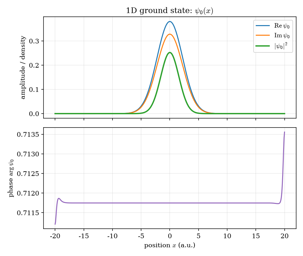
1d              static 1D spectrum and ground-state diagnostics
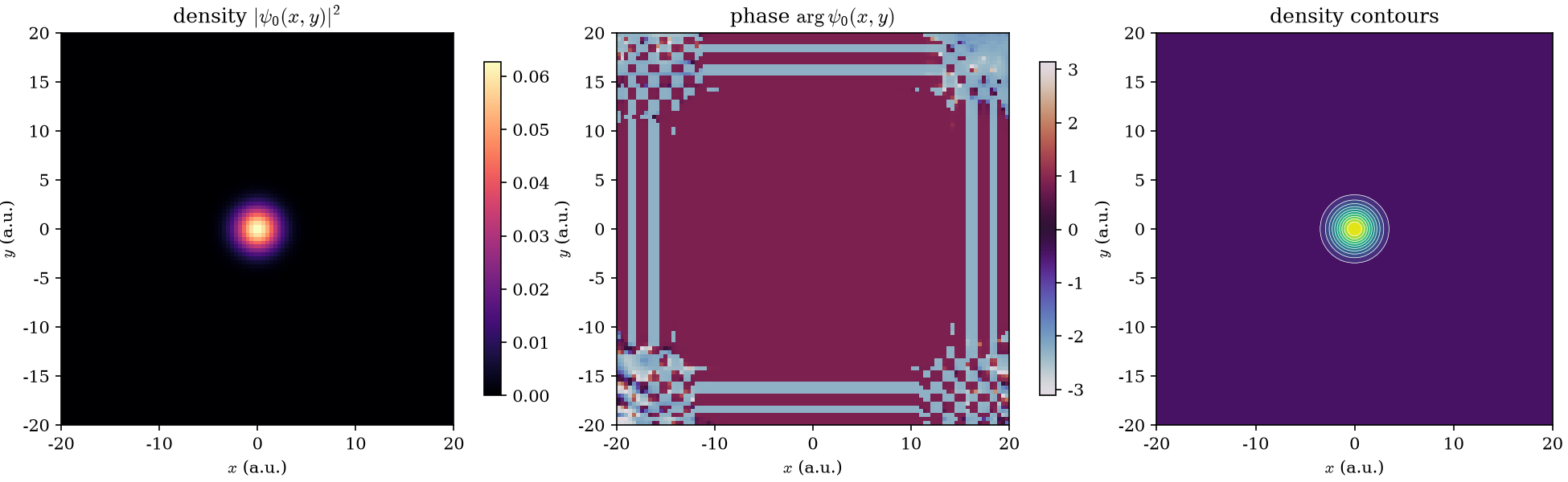
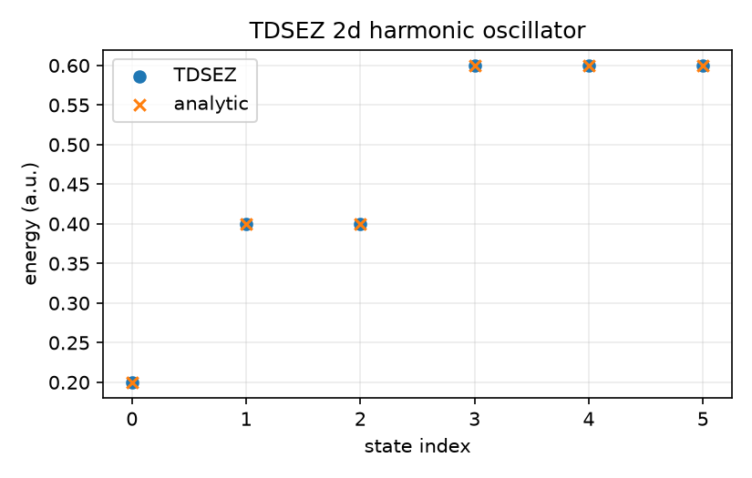
2d              static 2D spectrum, density, phase, and contours
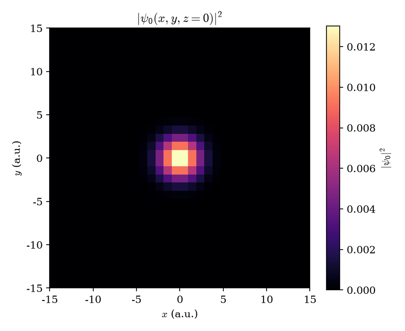
3d              static 3D reconstruction and central density slice
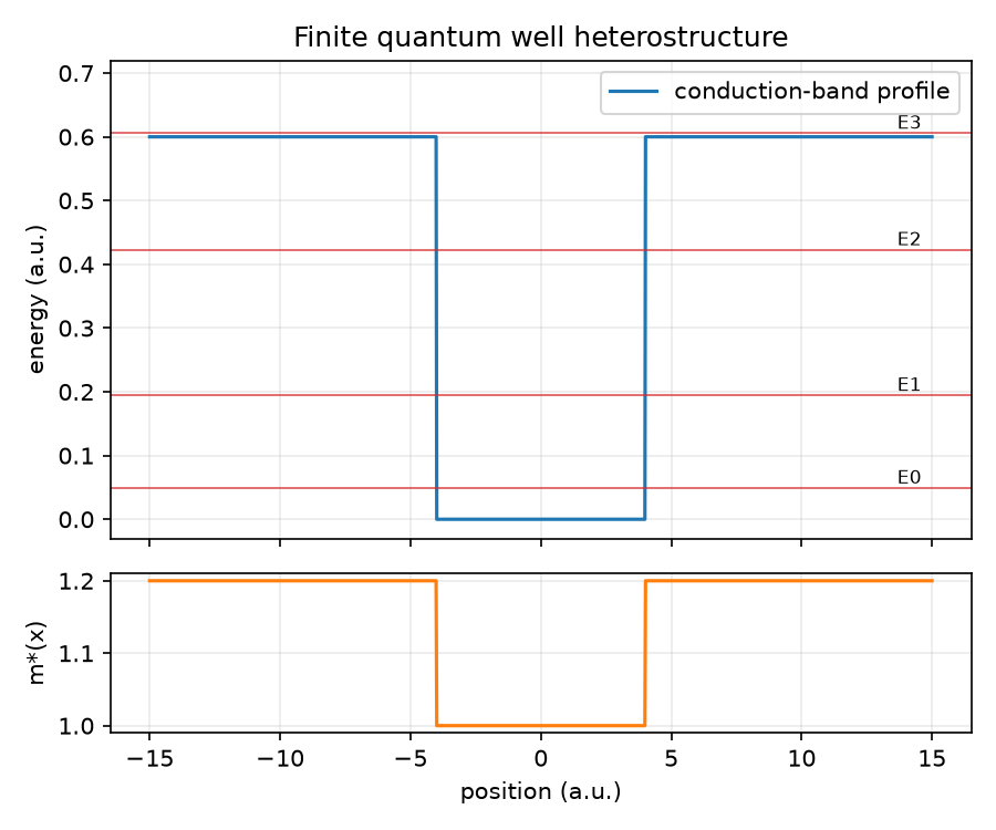
heterostructure finite quantum well with an effective-mass barrier
rabi            resonant driven dynamics
rabi-weak       weak resonant drive
rabi-detuned    off-resonant drive
rabi-suite      resonant, weak, and detuned comparison

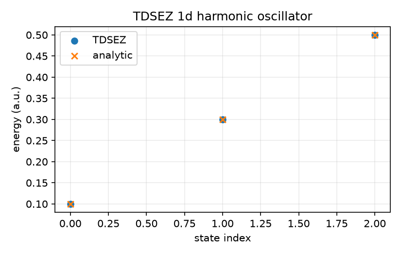
For the oscillator checks, the analytic references are

\[E_n^{(1D)} = \hbar\omega\left(n+\tfrac12\right), \qquad E_{n_x,n_y}^{(2D)} = \hbar\omega\left(n_x+n_y+1\right).\]

The 1D case also writes a ground-state diagnostic containing the real and imaginary components, probability density, and unwrapped phase. The 2D case writes density, phase, and filled contour views of the ground state. These plots are useful for checking parity, localization, nodal structure, and phase conventions before analyzing larger calculations.

The runner also includes a finite quantum-well heterostructure:

python examples/run_quick_examples.py --tdsez /tmp/tdsez-build/tdsez --case heterostructure

This example uses a 0.6 a.u. conduction-band offset outside -4 < x < 4 and a 20% larger barrier effective mass. It produces profile.csv and a potential_and_levels.png plot showing the band profile, effective mass, and computed bound-state energies.

Driven dynamics and Rabi-style transfer

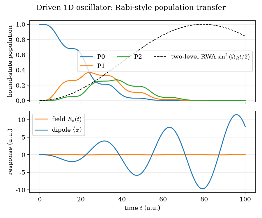
The rabi case starts in the harmonic-oscillator ground state and applies E_x(t) = 0.05 sin(0.2 t). The carrier is resonant with the 0-to-1 level spacing. Run it with:

python examples/run_quick_examples.py --tdsez /tmp/tdsez-build/tdsez --case rabi

The resulting rabi-populations-response.png contains bound-state populations, the applied electric field, and the dipole response. The CSV file contains those observables for further Fourier, susceptibility, or quantum-beating analysis.

The dashed curve is the analytic two-level rotating-wave estimate

\[P_1(t) \simeq \sin^2\!\left(\frac{E_0 |x_{01}| t}{4}\right), \qquad |x_{01}|=\sqrt{\frac{\hbar}{2m\omega}},\]

with E0 = 0.05 and omega = 0.2 in atomic units. The TDSEZ curves retain the full three-state dynamics, so their difference from this dashed reference shows where the two-level approximation breaks down.

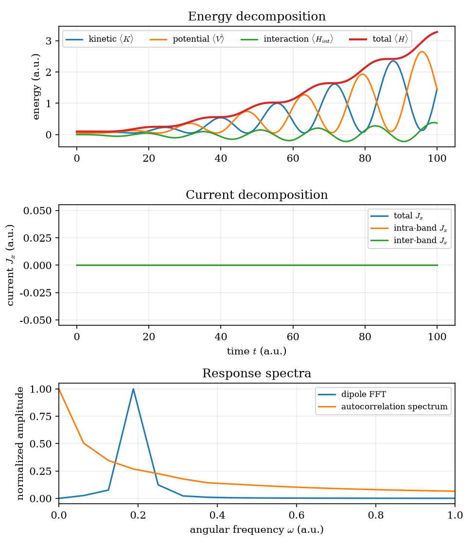
The runner also creates energy-current-spectra.png. It combines the kinetic, potential, interaction, and total energies; the intra-band, inter-band, and total currents; and normalized Fourier spectra of the dipole and autocorrelation. These are useful diagnostics for energy exchange, selection rules, and quantum beating.

Rabi-flopping suite

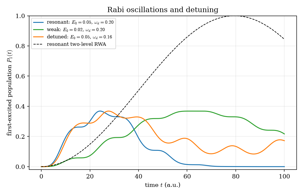
Use --case rabi-suite to compare three short 1D propagations:

• a resonant drive with E_0=0.05 and \omega_d=0.20;

• a weaker resonant drive with E_0=0.02;

• a detuned drive with E_0=0.05 and \omega_d=0.16.

Each run writes its own HDF5 observables and population plot. The suite also creates rabi-comparison.png, which overlays the first-excited-state population and the resonant two-level analytical reference. The detuned case shows the reduced transfer expected when the drive frequency is displaced from the transition energy.

python examples/run_quick_examples.py --tdsez /tmp/tdsez-build/tdsez --case rabi-suite

Reference spectra from this run:

Three-dimensional reconstruction

The 3d case uses eight cubic B-spline functions per axis and computes the ground state of an isotropic oscillator. Its analytical ground-state energy is E_000 = 3 hbar omega / 2 = 0.3 a.u.; the coarse smoke test returns approximately 0.3006 a.u. Run it with:

python examples/run_quick_examples.py --tdsez /tmp/tdsez-build/tdsez --case 3d

The runner reconstructs the three-dimensional field with the bundled evaluator and saves a central z=0 slice of |psi_0|^2.